Simulating Only What Changes: How to Recompute Elastic Wavefields Without Recomputing the Whole Model
Wave simulations appear in many fields, including earthquake science, seismic imaging, non-destructive testing, and medical ultrasound. The basic idea is straightforward: you specify a source—an earthquake, a pulse, or a transducer—and a model of the material, then compute how waves propagate, scatter, and eventually arrive at sensors in a 2D or 3D medium, producing synthetic data.
The challenge is that realistic models are large, and realistic wave physics is expensive to simulate. Even worse, many applications and processing workflows require not just one simulation, but hundreds or thousands of very similar ones. In imaging and inversion, for example, the model is updated repeatedly, often only within a small target zone each time. Running a full-domain simulation for every update is like re-rendering an entire movie scene because you moved one prop.
This story introduces the idea behind immersive wavefield modelling: a way to recompute wavefields after a local model change by simulating only a local region, while still reproducing the same result you would obtain from a full-domain simulation, including long-range interactions.
In practice, local wavefield modelling tries to balance two key goals:
- Speed: making repeated simulations much cheaper when only a small target zone changes.
- Accuracy: capturing wave interactions with the full exterior model, including waves that leave the local region and later return.
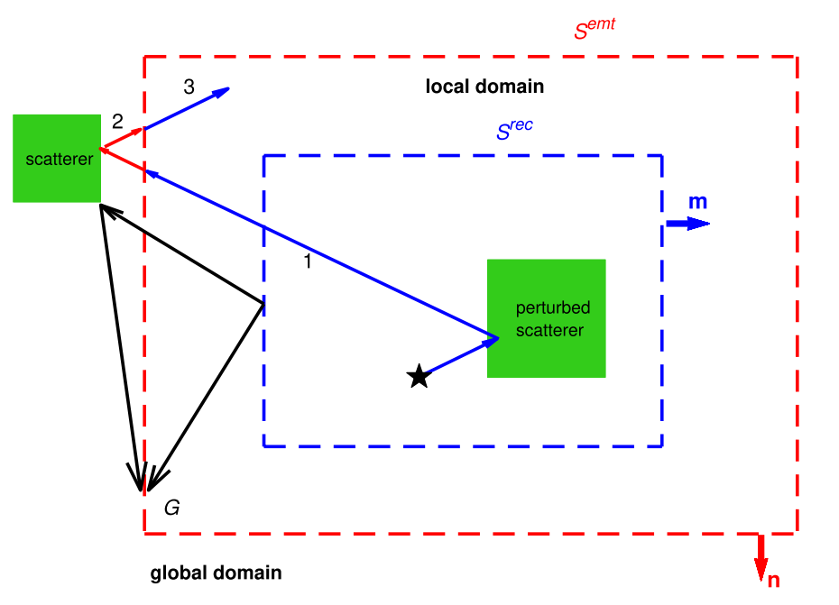
We simulate waves only inside the local box (red dashed line). A second surface (blue dashed line) records what the outside world would do. Precomputed responses describe how waves travel from the blue surface to the red one, allowing the boundary to inject the correct incoming waves and absorb outgoing waves. The small simulation then behaves as though it were still embedded in the full model.
Related: van Manen, Li, Vasmel, Broggini & Robertsson, Exact extrapolation and immersive modelling with finite-difference injection (2020).
Related: Li, Koene, van Manen, Robertsson & Curtis, Elastic immersive wavefield modelling (2022).
1) Why repeated wave simulations become painful
Many wave-modelling problems are not “one simulation” problems. Instead, they require solving the same wave equation over and over again for a family of models that are almost identical. This happens in full waveform inversion (FWI), in the design of wave-based imaging and monitoring surveys, and in sensitivity or uncertainty studies where many candidate models must be tested.
The expensive part is that each new run normally recomputes wave propagation through the entire computational domain, even when the actual model change is confined to a very small region. For example, an inversion update may alter properties only in a local target zone; a monitoring study may change only a damaged patch, a fluid-filled pocket, or a fracture corridor; and a design study may compare several versions of a small inclusion embedded in a much larger background medium. In all of these cases, most of the model stays the same, but a conventional simulation still pays the full global cost every time.
This is one reason local-domain modelling has become attractive in geophysics and beyond. The same basic computational pattern appears in several application areas:
- Seismic imaging and inversion: repeated updates inside a reservoir or target structure.
- Time-lapse monitoring: local changes caused by fluid movement, stress changes, or damage growth.
- Non-destructive testing: highly local defects such as cracks, voids, or fracture corridors inside a larger solid.
- Medical acoustics: wave interaction with a local organ or lesion inside the surrounding body.
- Electromagnetic/GPR modelling: local buried targets inside a much larger subsurface volume.
The obvious idea is therefore simple: if only a small subdomain changes, why not simulate only that subdomain? The difficulty is that waves do not respect our computational shortcuts. Energy can leave the local region, interact with the unchanged exterior, and later return. Those returned waves may themselves scatter again, producing higher-order long-range interactions between the target zone and the rest of the model. If a local method ignores those interactions, it may be fast, but it will not reproduce the true full-domain physics.
So the real challenge is not merely to make simulations smaller. It is to make a local simulation behave as though it were still embedded in the global model. That is exactly the problem immersive boundary conditions are designed to solve.
2) Conventional local replay: what it gets right—and what it can miss
Before immersive boundary conditions, a common way to speed up local recomputation was to use a record-and-reinject strategy. The idea is intuitive: if you already know how waves enter a target zone from the outside world, then perhaps you can replay that effect later without simulating the full model again.
In its simplest form, the workflow looks like this:
- Run a global simulation once in the original model.
- Record wavefields on a closed surface surrounding the target region.
- Modify the model inside that surface while keeping the exterior unchanged.
- Re-inject the recorded boundary wavefield so the local box receives the same incoming illumination as before.
This already gives a major practical benefit: instead of rerunning the whole domain, you only simulate the smaller region of interest. In many cases, that can save a great deal of time and memory.
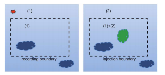
In the first simulation (left), the full model is used and the wavefield is recorded around a chosen boundary. In the second simulation (right), the model is changed only inside that boundary, and the previously recorded wavefield is injected back in. You can think of the final result as a combination of two parts: the original background response and the extra scattered response caused by the local change (the green object). This is a powerful and elegant use of superposition—but it is not yet a fully interactive connection to the outside world.
So what does this method get right? It correctly restores the incoming wavefield from the unchanged exterior and lets you study how a modified local target responds to it. That is why it has been very useful in wavefield separation, local modelling, and related finite-difference methods.
The limitation is more subtle. Once the target is changed, the new scattered waves do not simply stay inside the box. They can travel outward into the surrounding medium, interact with distant structures, and then return to the local region. Those returned waves may scatter again, and this process can repeat multiple times.
A conventional one-shot replay does not fully capture that two-way coupling between the local region and the rest of the model. In other words, it reproduces the original illumination well, but it does not naturally update the boundary to account for the new waves generated by the modified target and their later return from the exterior. That missing feedback is exactly what becomes important when higher-order, long-range interactions matter.
This is the gap that immersive boundary conditions are designed to fill: instead of replaying the boundary only once, they update it dynamically so that the local box remains coupled to the outside world throughout the simulation.
Related: Robertsson, van Manen, Schmelzbach, Van Renterghem & Amundsen, Finite-difference modelling of wavefield constituents (2015).
Related: van Manen, Li, Vasmel, Broggini & Robertsson, Exact extrapolation and immersive modelling with finite-difference injection (2020).
3) The core idea: Immersive Boundary Conditions (IBCs)
The main idea of Immersive Boundary Conditions (IBCs) is simple to state but powerful in practice: instead of simulating the whole model again, we simulate only a small local box around the region that changed, while making that box behave as though it were still embedded in the full medium.
You can think of it like filming a scene on a small studio set, but surrounding that set with screens and speakers that perfectly recreate the rest of the world. Inside the studio, everything still reacts as if the full environment were present. In wave modelling, the “screens and speakers” are the boundary conditions placed around the local domain.
What makes IBCs different from a simple one-time replay is that the boundary is not passive. It is an active boundary. At every time step, it does two jobs:
- It absorbs outgoing waves leaving the local box, so they do not reflect artificially from the numerical edge.
- It emits the correct incoming waves that the unchanged exterior model would send back into the box.
This matters because the local target and the exterior are constantly influencing each other. A wave may scatter from the modified region, travel out of the local box, interact with distant parts of the model, and then return later. In IBCs, those returning waves are not ignored. Instead, they are rebuilt at the boundary as the simulation runs, so the local model remains two-way coupled to the outside world.
In the elastic formulation developed in the paper, this is done using two nested surfaces:
- A recording surface inside the local domain, where the current wavefield is measured during the simulation.
- An emitting surface outside that recording surface, where boundary sources are applied.
The recorded wavefield on the inner surface is used to predict what should happen on the outer surface. In other words, the method takes what the waves are doing now on the recording surface and uses that information to update the boundary sources that represent the rest of the world.
That update is based on a set of precomputed wave responses in the unchanged background model. These responses are often described using Green’s functions, but in less mathematical language, you can think of them as a library of transfer rules: if the wavefield looks like this on one surface, what effect would the exterior model produce on the other surface?
The important practical feature is that this library is computed once in advance, before the local reruns begin. After that, it can be reused many times. So if you want to test many different local changes inside the target zone, you do not need to rebuild the full simulation each time. You keep the same surrounding world, reuse the same precomputed responses, and only change the local interior model.
This is why IBCs are so useful for repeated modelling. They let you keep the accuracy of a global simulation, but move most of the computation into a much smaller domain. In the ideal case, the wavefield inside the local box matches what a full-domain simulation would have produced, including complicated long-range scattering effects.
So the key message is: IBCs do not simply replay the boundary once—they continuously rebuild the influence of the outside world while the local simulation is running. That is what makes immersive modelling “immersive.”
4) Two practical ways to build the boundary: FD injection and MPS
Once the idea of immersive boundary conditions is clear, the next question is practical: how do we actually make this work inside a real wave simulator? In theory, the boundary around the local box should do two things at once. It should let waves leave the box without creating fake reflections, and it should also send back the waves that the surrounding medium would naturally return.
That sounds simple when described in words, but it is harder inside a numerical code. A wave simulator only knows about values on grid points, and in elastic modelling not all physical quantities are stored in the same place on that grid. So the boundary has to be not only physically correct, but also numerically consistent.
There are two main ways to do this:
- FD injection: the most precise approach, because it works directly with the finite-difference update rules.
- MPS (Method of Multiple Point Sources): a more compact and efficient approach, especially useful for elastic simulations.
4.1 FD injection: the exact route
FD injection starts from the way a finite-difference solver updates the wavefield. To update one grid point, the solver uses information from nearby points. This local pattern of neighbouring points is called a stencil. Now imagine that this stencil reaches across the boundary of the local box. If the outside world is no longer being simulated directly, then part of the information needed by the stencil is missing.
FD injection fixes exactly that problem. Rather than adding a general correction after the fact, it applies corrections precisely where the solver would otherwise notice that the exterior model is missing. In that sense, the method is built directly into the numerical scheme itself.
The figure below shows this idea visually. The local box is outlined, and the highlighted grid points are the ones that need special treatment because their update stencils cross the boundary.
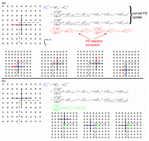
Only the grid points whose update stencils cross the boundary need special handling. That is why the method can be so accurate: it corrects the solver exactly where the missing exterior would matter.
Another way to think about FD injection is this: it tells the local simulation exactly what the missing outside world would have contributed at those boundary-adjacent points. If everything is done consistently, the local simulation can reproduce the same wavefield that a full-domain run would produce inside the box.
This makes FD injection a very useful reference method. When the setup is fully consistent with the numerical solver, it can match the full simulation to machine precision. In other words, any difference becomes so small that it is essentially just numerical roundoff.
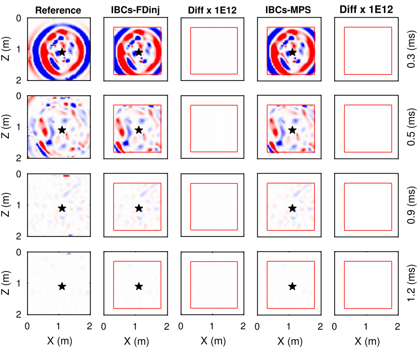
The acoustic examples below show a demanding test case with strong reflections and scattering. This is important, because a boundary method is only convincing if it still works when the wavefield becomes complicated.
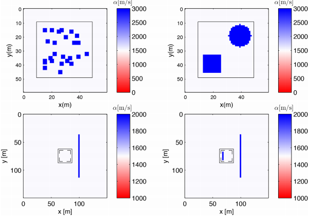
The model includes strong scatterers and multiple wave interactions, making it a good stress test for local immersive modelling.
The cleanest test is simply to compare the local result with a full-domain simulation. If the two wavefields are the same, then the local box is successfully behaving as if it were still embedded in the large model.
The difference images are enlarged dramatically to make tiny residuals visible. In practice, the local and full-domain results are nearly indistinguishable.
The trade-off is that FD injection can become expensive. To keep the simulation exact, the method has to track many boundary-related values, evaluate correction terms, and store a large amount of precomputed response information.
This becomes more costly when the finite-difference stencil gets wider. A wider stencil reaches farther across the boundary, so more grid points need correction. That means more memory, more bookkeeping, and more computation.
In short: FD injection is the most exact option, but it can become heavy for large or higher-order simulations.
Related: van Manen, Li, Vasmel, Broggini & Robertsson, Exact extrapolation and immersive modelling with finite-difference injection (2020).
4.2 MPS: a lighter and more flexible route
FD injection is very powerful, but elastic waves make everything more complicated. In elastic modelling, we do not track just one quantity. We usually track particle velocities and stresses, and these may be stored at different locations on a staggered grid. That makes boundary recording and injection more delicate than in the simpler acoustic case.
This is where MPS, short for Method of Multiple Point Sources, becomes attractive. Instead of correcting many individual stencil-crossing grid points, MPS represents the boundary effect using many small point sources arranged around the local box.
A helpful mental picture is to imagine a ring of tiny speakers around the boundary. Each source on its own is simple, but together they recreate what the surrounding medium would send back into the box. That gives a much more compact boundary treatment.
The figure below shows why this needs some care in elastic modelling: the wavefield components do not all live at the same grid locations, so recording and reinjecting them consistently is not just a matter of reading and writing one value per point.
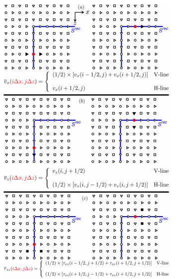
The idea is simple, but the implementation is subtle because different elastic variables are stored at different grid positions.
One especially tricky part is the corners of the boundary. Corners are where simple boundary treatments often struggle, because waves can approach them from multiple directions and different wavefield components meet there in awkward ways.
The setup below shows the basic immersive modelling geometry for the elastic case. Only the local box is simulated directly, while the recording and emitting surfaces keep that box connected to the rest of the model.
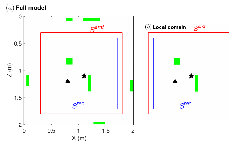
The simulation runs only inside the local box, while the surrounding boundary machinery makes that box behave as if the exterior model were still present.
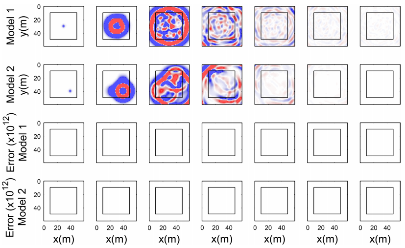
In a basic second-order elastic scheme, both FD injection and MPS can recover the same result as the full simulation to machine precision. That is important because it shows MPS is not just a rough shortcut in this setting: it can be just as accurate while using a simpler boundary representation.
The difference images are scaled up to reveal tiny residuals. In practice, both local simulations closely reproduce the full solution.
So why use MPS at all if FD injection is also exact? The answer is simple: efficiency. In repeated local simulations, much of the cost comes from the boundary treatment itself. With FD injection, the number of boundary-related points grows as the stencil gets wider. That growth quickly increases storage and runtime.
MPS avoids much of that expansion. Its boundary description stays more compact, which makes it much more attractive when you need to run many simulations or when the elastic solver becomes more sophisticated.
In higher-order schemes, MPS is no longer perfectly exact, but it often remains very accurate. The remaining mismatch is usually small and tends to be concentrated near the boundary, especially around corners.
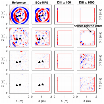
The visible differences are small and mainly concentrated near the boundary, while the overall wavefield remains very close to the full-domain result.
So the practical takeaway is:
- FD injection is the most exact and reliable option when you want the boundary treatment to match the solver as closely as possible.
- MPS is the more efficient option, and it can still be extremely accurate while using a much lighter boundary representation.
If I had to summarize the difference in one sentence: FD injection is the precision-first method, while MPS is the efficiency-first method for repeated local wave simulations.
Related: Li, Koene, van Manen, Robertsson & Curtis, Elastic immersive wavefield modelling (2022).
5) So what does the workflow actually look like?
Immersive modelling is especially useful when you need to test many local changes without rerunning the whole model every time. The basic strategy is to do the expensive global preparation once, and then reuse that information for much cheaper local simulations.
A typical workflow looks like this:
- Choose a target zone: draw a box around the part of the model you expect to change.
- Precompute the exterior response once: use the unchanged background model to work out how the surrounding medium should affect the box boundary.
- Run local simulations: each time the target region is updated, simulate only that small box while the boundary reproduces the effect of the rest of the model.
- Use the results: inside the box, and at your receivers, the simulation behaves as if the full domain had been recomputed.
In short, the workflow is all about reusing what does not change, so that you only spend time recomputing what does change.
6) When does immersive modelling really make sense?
Immersive modelling is powerful, but it is not always the right tool. It works best when your problem has a very particular shape: a large background model that stays the same, and a small target region that changes many times.
That usually means it is most worth using when:
- The update is local: only a small part of the model changes between runs.
- You need lots of reruns: for example, in inversion loops, monitoring studies, or testing many candidate scenarios.
- The outside world still matters: waves interact with the surrounding medium and those interactions need to be preserved.
In contrast, the method becomes less appealing when the problem is global rather than local. If large parts of the model are changing, or if you only need a single simulation, then the extra setup may not be worth the effort. Memory can also become a practical limitation, because the exterior responses must be stored somewhere.
So the short version is: immersive modelling pays off when you want to recompute a small changing region many times without losing the influence of the larger unchanged model.
7) Why this idea matters beyond one method
What makes immersive modelling interesting is that it is not just a clever boundary trick. It reflects a much broader pattern that appears in many wave problems: a large background stays mostly the same, while only a small region changes.
Once you look at problems that way, the value of the method becomes much clearer. Instead of recomputing the whole world every time, you focus the expensive work only where something has actually changed, while still keeping the influence of everything outside.
That basic idea shows up in many different settings:
- Seismic imaging and inversion: update a reservoir or target area many times without rerunning the full subsurface model from scratch.
- Time-lapse monitoring: track local changes caused by fluid movement, stress redistribution, or damage over time.
- Non-destructive testing: model waves around a suspected crack or defect while still accounting for the rest of the structure.
- Medical acoustics: study how waves interact with a local organ, tumour, or lesion without losing the surrounding body context.
- Laboratory wave experiments: connect a real physical sample to a simulated exterior so the experiment behaves as if it were part of a larger world.
So the bigger message is simple: when only a small part of a system changes, we should not have to recompute everything from the beginning. Immersive modelling offers one way to make that idea practical for wave simulations.
References
- Robertsson, J., van Manen, D.-J., Schmelzbach, C., Van Renterghem, C., & Amundsen, L. (2015). Finite-difference modelling of wavefield constituents, Geophysical Journal International. https://doi.org/10.1093/gji/ggv379
- van Manen, D.-J., Li, X., Vasmel, M., Broggini, F., & Robertsson, J. (2020). Exact extrapolation and immersive modelling with finite-difference injection, Geophysical Journal International. https://doi.org/10.1093/gji/ggaa317
- Li, X., Koene, E., van Manen, D.-J., Robertsson, J., & Curtis, A. (2022). Elastic immersive wavefield modelling, Journal of Computational Physics, 451, 110826. https://doi.org/10.1016/j.jcp.2021.110826