Listening to Rocks' Breathe: A View of Nonlinear Elasticity in Granular Solids
When we’re first taught elasticity, we usually meet Hooke’s law: double the stress, double the strain. Springs behave nicely, waves pass through without changing shape, and everything stays linear and predictable.
Real rocks don’t play by those rules. Sandstones, chalk, concrete, and crushed fault rocks are made of tiny grains and cracks (see picture below). At their contacts, grains are constantly opening, closing, and slipping past each other as the rock is shaken or stressed. At small vibrations they act almost linearly, but once we shake them a bit harder – at levels similar to strong seismic waves – they start to show a very different, “nonlinear” personality.
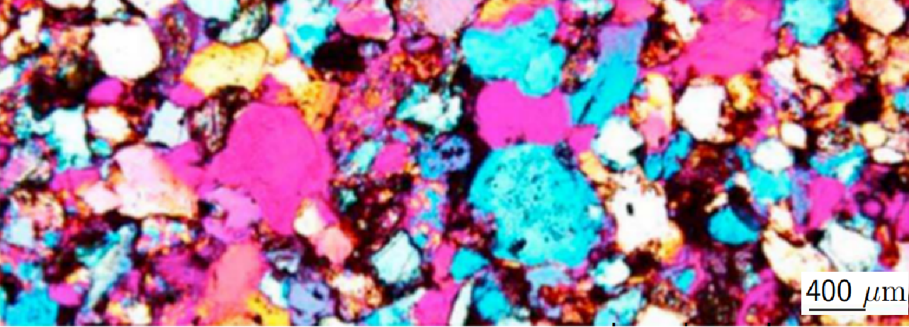
Each grain touches its neighbours at tiny, fragile contacts – the source of much of the rock’s nonlinear behaviour. Field of view: 3.1 mm. Adapted from Rivière et al. (2015b).
Over the last few decades, lab experiments have shown that granular rocks behave in surprisingly complicated ways once we drive them hard enough with seismic‑like vibrations. Their resonant frequencies shift as the drive increases, their stiffness can drop almost instantly when we change the load, and then recover only very slowly. Their response also “remembers” what happened before: it depends on the history of the deformation, not just what we are doing to the sample right now.
One of the simplest ways to see this is to put a rock sample in a resonance experiment, turn up the shaking, and watch how its favourite vibration frequency moves. In a linear world, the resonance peak would simply get taller as we shake harder, but its frequency would stay put. In the lab, we see something else entirely as below.
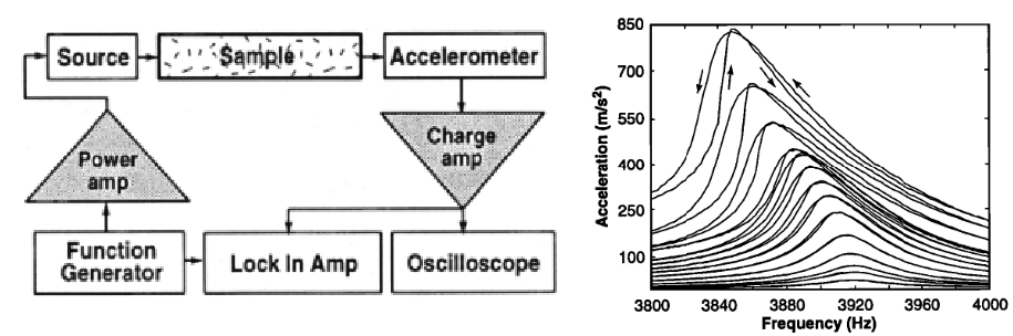
(Left) Sketch of a typical resonance setup: a rock bar is driven at one end and its motion is measured at the other. (Right) Resonance curves for Berea sandstone as the drive amplitude is increased. At low amplitudes, the peak is nearly symmetric and stays at the same frequency. At higher amplitudes, the peak shifts, sharpens, and becomes asymmetric – a clear sign of nonlinear behaviour. Adapted from TenCate & Shankland (1996).
To dig deeper into this behaviour, laboratory researchers have combined two operations:
- Drive the rock in resonance to create controlled, relatively large strains, and
- Probe its stiffness with small, high‑frequency waves while it is being shaken.
This is what Dynamic Acousto‑Elastic Testing (DAET) and Nonlinear Resonant Ultrasound Spectroscopy (NRUS) do:
- NRUS: track the resonance peak as drive increases.
- DAET: monitor high‑frequency wave speed during low‑frequency pumping and recovery.
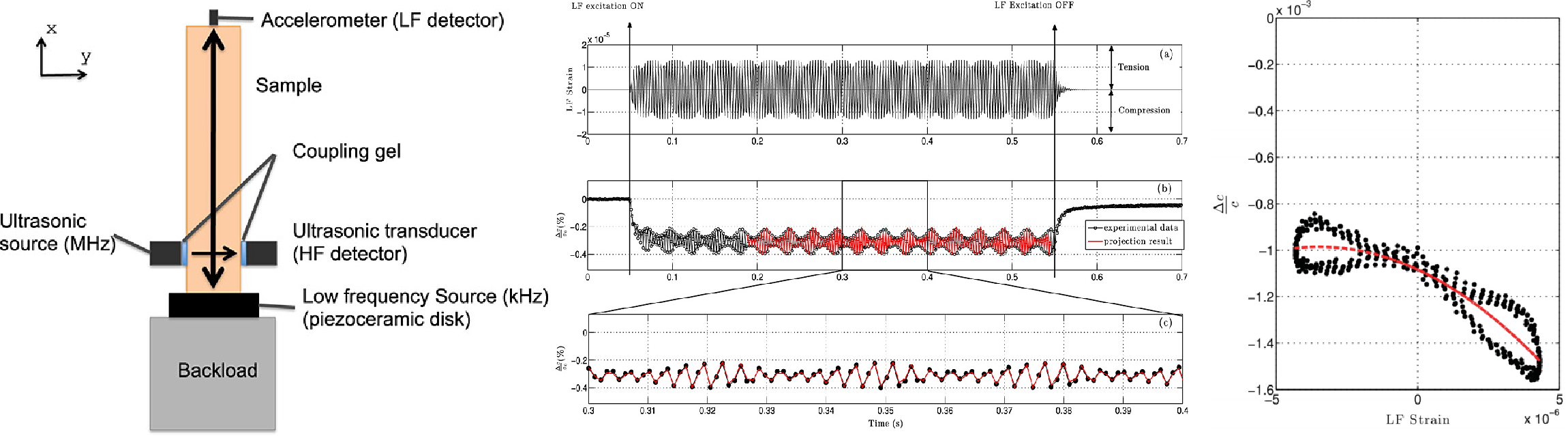
(Left) DAET setup: a low‑frequency (kHz) drive excites the first compressional resonance at strains of about $ 10^{-7} $–$ 10^{-5} $, while 1 MHz pulses probe the instantaneous seismic velocity. (Middle)Example of projecting the high‑frequency velocity changes onto the low‑frequency strain cycle. (Right) The resulting nonlinear “loop” shows hysteresis and conditioning – the rock’s stiffness does not follow the same path on loading and unloading. Adapted from Rivière et al. (2015a).
Another striking feature is that rocks can take a very long time to recover after being strongly shaken. If we “condition” a sample by driving it hard for a while, its seismic velocity drops. When we stop shaking, the velocity does not bounce back right away. Instead, it creeps back logarithmically with time – fast at first, then slower and slower, over minutes to hours:
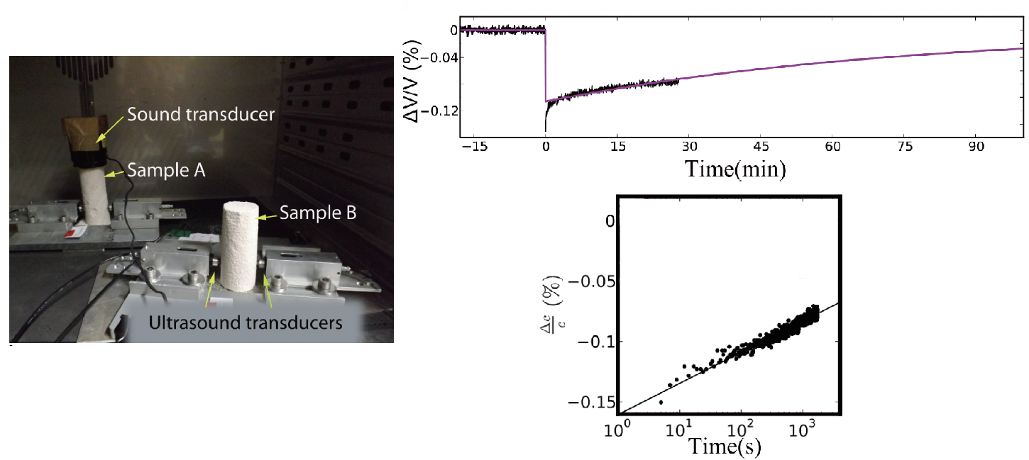
(Left) Experimental setup to monitor seismic velocity during and after a resonance experiment. (Right) After strong shaking (“conditioning”), the seismic velocity in gypsum recovers slowly, following an seemingly logarithmic trend with time rather than a simple exponential. Adapted from Gassenmeier (2015).
This is not just a lab curiosity. At the scale of real faults and basins, the shallow crust shows very similar behaviour after strong earthquakes. Immediately after a big event, seismic velocities in the upper crust drop measurably; in the weeks to years that follow, they gradually climb back toward their pre‑event values. Noise‑based monitoring of the Parkfield segment of the San Andreas Fault is a good example as below.
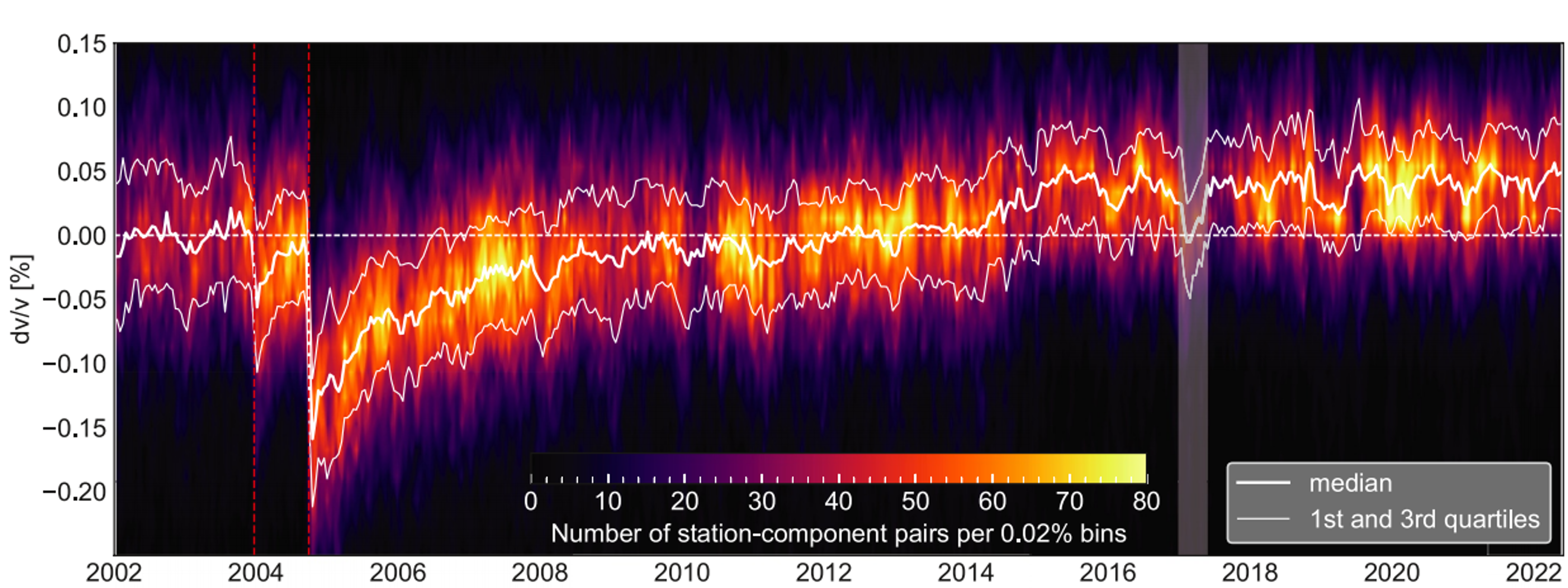
Background colormap shows how often a given dv/v value is observed in each time bin; the thick line is the median, and thin lines mark the quartiles. The San Simeon (SS) and Parkfield (PF) earthquakes (red dashed lines) reduce seismic velocity, followed by a slow recovery over months to years – echoing the slow dynamics seen in the lab. Gray shading marks a period affected by clock drift. Adapted from Okubo et al. (2024).
My research is about building a simple, thermodynamics‑based contact model that can reproduce all of above behaviours in a unified way.
Related: Xun Li, A unified interpretation of nonlinear elasticity in granular solids – Master’s thesis, Colorado School of Mines.
1) Why Rocks (Sometimes) Don’t Obey Hooke’s Law
Hooke’s law says that stress is proportional to strain as long as deformations remain “small”. That works well for many engineering materials, and it underpins most of exploration and global seismology: we model seismic waves as small perturbations travelling through a linear elastic Earth.
Granular solids (e.g., sandstone, concrete, fault gouge, porous chalk) behave differently from homogeneous solids. They comprise stiff mineral grains cemented by weaker phases and contain abundant internal defects—microcracks, grain contacts, and intergranular bonds. Although these features are small (nanometres to microns), they are numerous and typically control bulk compliance and wave attenuation. A compressed pack of glass beads is also a granular material: under sufficient confinement it develops solid-like behaviour governed primarily by contact mechanics. Below shows representative X-ray micro-CT slices of two granular solids imaged in situ under triaxial loading.
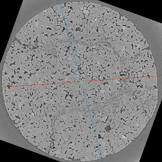
Bright regions correspond to mineral grains; dark regions are pores. Pore space and grain contacts form compliant “weak links” that commonly localise damage and influence nonlinear elasticity and attenuation.
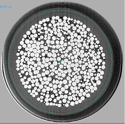
The near-spherical grains and well-defined contacts provide a controlled analogue for isolating contact mechanics and interpreting nonlinear and hysteretic behaviour. Image courtesy of Dr. Alexis Cartwright Taylor and Michael Chander (University of Edinburgh).
The key point is that “small strain” at the sample scale does not mean small deformation everywhere inside the microstructure. Even when the bulk strain is only microstrain, deformation can concentrate at a tiny fraction of the volume: at compliant pores, crack tips, and fragile grain contacts (Guyer and Johnson, 2009). Those contacts can open/close or slip in an asymmetric, history dependent way—so the effective stiffness depends on both the instantaneous strain and how the sample got there.
A large body of classic experiments has established a few robust features of granular and cracked solids:
- Nonlinearity appears at surprisingly small strains—sometimes as low as $ 10^{-7} $–$ 10^{-6} $—well below the level where conventional lattice anharmonicity would be expected to dominate.
- The stress–strain relationship exhibits hysteresis and memory as shown above in the Introduction. The response is highly asymmetric: loading and unloading follow different paths, and the current response depends on the material’s previous strain history. Compression tends to close cracks and stiffen the material, whereas tension can open contacts and trigger pronounced softening.
2) Mathematical Playground: The Duffing Oscillator
Before getting lost in the messy microstructure of real rocks—thousands of contacts, partial slip, crack opening/closure, and long-term “memory”—it helps to study a clean nonlinear system that already reproduces one of the most visible lab signatures: a resonance peak that tilts and develops a “cliff”.
The block position follows the numerical solution $ x(t) $ of the forced Duffing equation. The spring drawing is only a visual guide (not a force-law plot): the key idea is that the restoring force includes a cubic term, so the “effective stiffness” depends on amplitude—one of the simplest routes to tilted, asymmetric resonance peaks and jump (“cliff”) behaviour in frequency sweeps. (Example parameters in this animation: φ=0.1, k=0.2, δ=0.55, $ A_r $=0.75, ω=1.0)
The simplest playground for this is the Duffing oscillator. You can picture it as a mass-on-a-spring system as shown above, where the spring is no longer perfectly linear: as the motion grows, the restoring force becomes slightly stronger or weaker than Hooke’s law would predict.
$ \ddot{x} + \phi \dot{x} + kx + \delta x^3 = A_r \sin(\omega t). $
In this equation, $ x $ is the displacement (or a strain-like variable), $ \phi $ controls damping (energy loss), $ k $ is the familiar linear stiffness, and the cubic term $ \delta x^3 $ introduces nonlinearity. The system is driven at frequency $ \omega $ with amplitude $ A_r $.
The sign of $ \delta $ sets the “personality” of the oscillator:
- Softening ($ \delta < 0 $): the effective stiffness drops as amplitude increases, so the resonance shifts to lower frequency.
- Hardening ($ \delta > 0 $): the effective stiffness increases with amplitude, so the resonance shifts to higher frequency.
Even though the drive is sinusoidal, the response amplitude depends on frequency and on how large the oscillation becomes, because stiffness is amplitude-dependent.
The most revealing view is the frequency response: sweep $ \omega $ and track the steady oscillation amplitude. In a linear oscillator the resonance peak is smooth and symmetric. In the Duffing oscillator, as $ | \delta | $ or $ A_r $ grows, the peak shifts and leans—already resembling what we see in many rock resonance experiments.
If the nonlinearity is strong enough (especially for softening), the curve can actually fold over. That folding implies that, for the same driving frequency, there may be more than one possible steady response. In a sweep experiment the system follows one stable branch until it reaches the fold, then it jumps abruptly to another branch—creating the vertical-looking “cliff” where tiny frequency changes produce large amplitude changes.
As the response grows, the peak becomes asymmetric and shifts (for softening, toward lower frequency).
Once the curve folds, sweeps can jump between stable branches, producing sharp amplitude changes.
The above mathematical oscillator actually connects back to rocks: the Duffing oscillator is a clean way to understand why nonlinear resonance curves naturally become skewed and can develop cliffs—even without any microcracks, friction, or complex geometry. But real granular rocks go further: they show pronounced hysteresis, conditioning, and slow recovery that a basic Duffing model does not capture. The next step is to move from “one nonlinear spring” to a physically motivated model for many evolving grain contacts.
Related: Xun Li, A unified interpretation of nonlinear elasticity in granular solids – Master’s thesis, Colorado School of Mines.
3) Thermodynamic Picture: Fractures as Bistable Elements
The Duffing oscillator is a great “shape of nonlinear resonance” toy model, but it is essentially instantaneous and memoryless. The thermodynamic contact picture here adds what rocks seem to need most: internal state variables (open/closed populations) with rate-dependent evolution.
The key idea is to stop thinking of a rock as “one spring”, and instead treat it as many tiny mechanical switches. Each grain contact (or microcrack) can sit in one of two metastable states: a closed state (stiffer) or an open state (softer), as shown below.
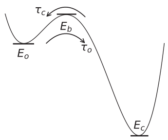
Each contact has two states (open/closed) separated by an energy barrier; thermal activation enables switching.
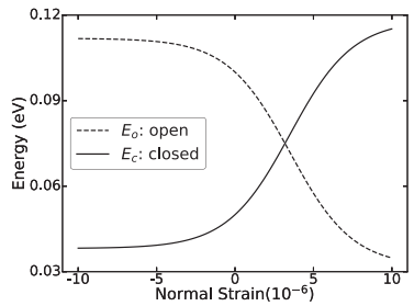
Sigmoid dependence on strain makes opening favoured in extension and closing favoured in compression, while keeping the model smooth and stable for numerical simulation.
Between those states sits an energy barrier $ E_b $ (left panel above ). On its own, a contact would prefer to remain in whichever state is currently lower in energy. But thermal fluctuations (“molecular jiggling”) occasionally kick the contact over the barrier—so the contact can switch between open and closed. This is the same statistical-physics logic used for many activated processes (chemical reactions, diffusion over barriers, etc.).
In this model, switching times are Arrhenius:
$$ \tau_o = A \\, e^{(E_b - E_o)/(k_B T)}, \quad \tau_c = A \\, e^{(E_b - E_c)/(k_B T)}. $$
Here $ \tau_o $ is the characteristic time for a closed contact to open, and $ \tau_c $ for an open contact to close. Because of the exponential, small changes in energy produce huge changes in switching rate—one reason why rocks can become nonlinear at surprisingly tiny strains.
For contacts sharing the same barrier energy $ E_b $, the fraction of open contacts $ n_o(t) $ evolves as:
$$ \frac{d n_o}{dt} = - \frac{n_o}{\tau_o} + \frac{1 - n_o}{\tau_c}, \quad n_{\mathrm{eq}} = \frac{1}{1 + \exp\big[(E_o - E_c)/k_B T\big]}. $$
The equilibrium fraction $ n_{\mathrm{eq}} $ is a smooth, thermodynamic “target” set by the energy difference $ E_o - E_c $. Dynamics come from the fact that the system does not instantly reach equilibrium—it relaxes toward it with a rate controlled by $ \tau_o $ and $ \tau_c $.
3.1) How strain tilts the landscape
Shaking the rock changes stresses at contacts. In the model, that effect enters by letting the state energies depend smoothly on the dynamic strain $ \varepsilon $ using sigmoid functions:
$$ E_o(\varepsilon) = B_0 - \frac{A_1}{1 + \exp[-(\varepsilon - \mu)/\sigma]}, \quad E_c(\varepsilon) = A_0 + \frac{A_1}{1 + \exp[-(\varepsilon - \mu)/\sigma]}. $$
You can read these curves in plain language:
- When the strain becomes more extensional, the open state becomes energetically favourable: more contacts want to open.
- When strain becomes more compressional, the closed state becomes favourable: more contacts want to close.
- The transition is not a sharp “on/off”. The sigmoid makes it gradual, reflecting the fact that contacts are diverse and local geometries vary.
3.2) From one timescale to many: why recovery can look logarithmic
A single barrier $ E_b $ would produce one characteristic relaxation time (roughly exponential recovery). Real rocks, however, contain an enormous variety of contact geometries and microcrack sizes—so we assume a spectrum of barrier energies, here taken as uniform on $ E_b \in [E_{b,\min}, E_{b,\max}] $. Averaging over this population gives a sample-scale open fraction $ N_o(t) $.
This broad collection of relaxation times is one of the cleanest routes to “slow dynamics”. Intuitively: after strong shaking, the fast contacts snap back quickly, but the slow contacts keep relaxing for a long time. When you add up lots of exponentials with many timescales, the net recovery can resemble a logarithm over a broad time window. In simplified form:
$$ \Delta Y(t) \propto - \int_{\tau_{\min}}^{\tau_{\max}} \frac{d\tau}{\tau}\, e^{-t/\tau} \;\approx\; - \log t \quad (\tau_{\min} \ll t \ll \tau_{\max}). $$
That’s the “physics shortcut” behind the famous lab observation: quick recovery at first, then slower and slower, without a single clean time constant.
3.3) Turning contact state into a measurable stiffness
We connect contact statistics to bulk stiffness with a simple linearized damage law:
$$ Y(t) = Y_0 - C_0 \big( N_o(t) - N_{\mathrm{ori}} \big). $$
In words: if more contacts are open (larger $ N_o $), the sample is softer (smaller $ Y $). Since resonance frequency scales roughly like the square root of stiffness, even modest changes in $ Y $ can produce measurable resonance shifts:
$$ f(t) \approx f_0 \sqrt{\frac{Y(t)}{Y_0}}. $$
This closes the feedback loop: strain $ \rightarrow $ energies $ \rightarrow $ switching $ \rightarrow $ $ N_o(t) $ $ \rightarrow $ stiffness $ Y(t) $ $ \rightarrow $ strain, as summarized in the feedback cycle as below! And because switching is rate-dependent, the stiffness depends on history—not just the instantaneous strain.
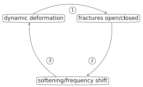
Dynamic strain biases contact energies, contacts switch over barriers, the open fraction changes stiffness, and stiffness feeds back into the deformation—naturally producing amplitude dependence, hysteresis, and slow recovery.
Reference: Li, X., Sens‑Schönfelder, C. & Snieder, R. (2018), Physical Review B.
4) Simulating Real Resonance Experiments
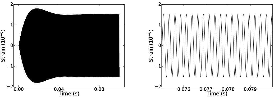
Lab resonance experiments are not just “measure a curve once and you’re done”. They are more like slowly tuning a radio dial: you pick a driving frequency, hold it for a short time, record how strongly the sample responds, then step to the next frequency and repeat. If the rock’s internal contacts are evolving while you do this, the curve you measure is partly shaped by the measurement process itself.
4.1) One resonant mode + a stiffness that can change with time
To mimic a resonance-bar experiment without simulating every grain, the thermodynamics‑based model keeps only a single resonant mode (think: “the main way the bar likes to vibrate”) and tracks its modal amplitude $ R_A(t) $. The key twist is that the natural frequency is not constant: it depends on the evolving Young’s modulus $ Y(t) $ from the contact model in Section 3.
$$ \ddot{R}_A + 2\gamma \dot{R}_A + \Omega^2(t)\,R_A = A_r \, e^{-i\omega t}, \quad \Omega(t) = \frac{\pi}{L_0}\sqrt{\frac{Y(t)}{\rho}}. $$
Here $ \gamma $ is damping, $ \omega $ is the driving frequency, $ L_0 $ is the sample length, and $ \rho $ is density. If $ Y(t) $ drops (more contacts opening), then $ \Omega(t) $ drops too—so the “centre” of the resonance peak can drift while you are measuring it.
4.2) Experimental protocol: “hold, measure, step”
The simulation follows the same protocol used in NRUS/DAET-style frequency sweeps:
- Choose a frequency $ \omega $ and drive the sample there.
- Hold that frequency for a finite dwell time $ \Delta t $. During this hold, the oscillator responds and the internal state $ N_o(t) $ evolves, changing $ Y(t) $.
- Measure the response amplitude (often reported as an acceleration-like quantity proportional to $ \omega^2 R_A L_0 $).
- Step the frequency by $ \Delta f $ and repeat, sweeping upward or downward.
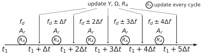
At each frequency the system is driven for a dwell time $ \Delta t $ before stepping by $ \Delta f $. Because the internal state evolves during every hold, the resonance curve is an outcome of both mechanics and kinetics (how fast contacts can switch).
A subtle but crucial point: the final internal state at one step becomes the initial state for the next. That is how the model naturally builds in memory and explains why up-sweeps and down-sweeps can differ.
4.3) “Clock” inside the rock: the slowest contacts set $ \tau_{\max} $
The thermodynamic contact model contains many relaxation times (because we include many barrier energies $ E_b $). The slowest ones dominate long-term memory. A convenient definition is the maximum relaxation time $ \tau_{\max} $, set by the largest barrier $ E_{b,\max} $:
$$ \tau_{\max}^{-1} = \left(\tau_o^{-1}+\tau_c^{-1}\right)\big|_{E_b = E_{b,\max}} $$
This gives an intuitive way to think about sweep speed:
- Fast sweep: $ \Delta t \ll \tau_{\max} $. The rock cannot fully “catch up” at each step, so the measured curve depends strongly on history (strong memory, larger up–down differences).
- Slow sweep: $ \Delta t \gg \tau_{\max} $. The contact population nearly equilibrates at each frequency, so the curve is closer to a quasi-steady response (weaker memory, smaller up–down differences—unless bifurcations appear).
With this setup, we can now do something very close to what experimentalists do: run the same sweep twice (up and down), change the drive amplitude, change the sweep rate, and ask: what features come from “instantaneous nonlinearity” and what features come from slow, history-dependent contact evolution?
5) What the Model Reproduces: Slow Dynamics, Asymmetry, Hysteresis, and Cliffs
Now comes the fun part: once we connect “many switchable contacts” to a resonance experiment protocol (Section 4), we can run the same measurements people do in the lab—just inside a computer. Below, we show model output (left) with a matching lab observation (right) if found from literature.
5.1 Slow Dynamics: why recovery looks like a straight line on a log-time plot
First, the signature that surprised many people when it was discovered: after strong shaking (“conditioning”), the rock does not bounce back immediately. Its stiffness (and therefore resonance frequency) recovers slowly— often close to a straight line when plotted against $ \log t $.
In the model, this happens naturally because we have many contacts with many barrier energies. Some contacts switch back quickly; others are “stuck” behind larger barriers and relax much more slowly. Add up that whole population and you get a long-tailed recovery that can look logarithmic over a wide time window.
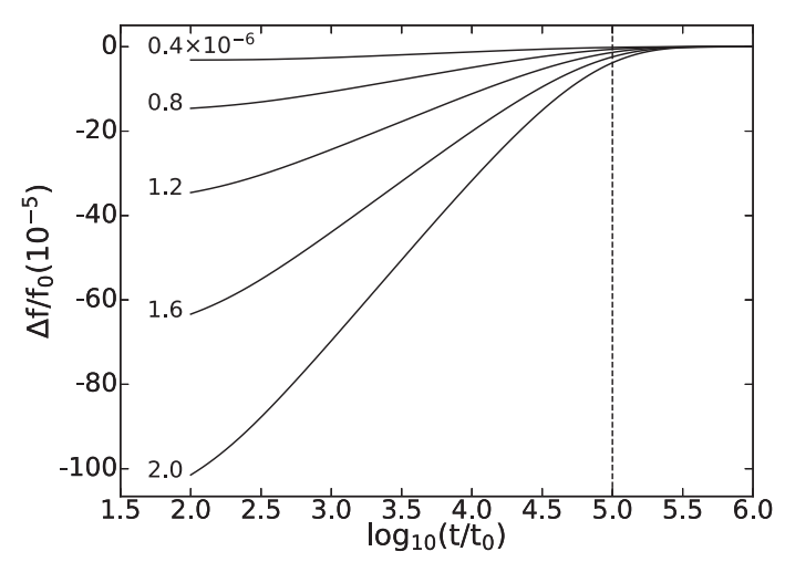
After conditioning, the resonance frequency recovers roughly linearly with $ \log t $ over decades in time.
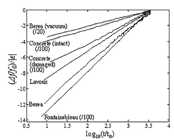
Strong shaking reduces wave speed; recovery is slow and often close to logarithmic in time. Figure adapted from TenCate et al., (2000).
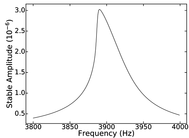
5.2 Asymmetric resonance curves: why the peak “leans”
Next, the resonance peak itself. In a perfectly linear material, the resonance curve is symmetric. In granular rocks it often becomes skewed—one side of the peak steepens and the other side spreads out.
The model explanation is simple in words: the sample softens most strongly near resonance (because that is where the strain amplitude becomes largest). So while you are measuring the peak, the modulus $ Y(t) $ is drifting downward and the natural frequency $ \Omega(t) $ is moving too. That “moving target” makes the measured curve asymmetric.
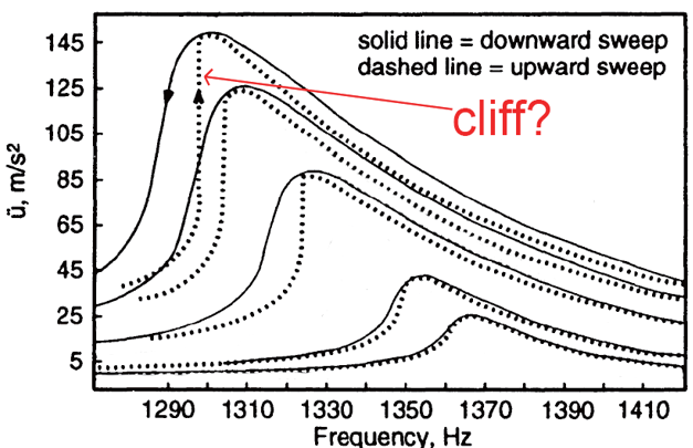
As drive increases, the peak shifts and becomes asymmetric because the stiffness is evolving during the sweep.
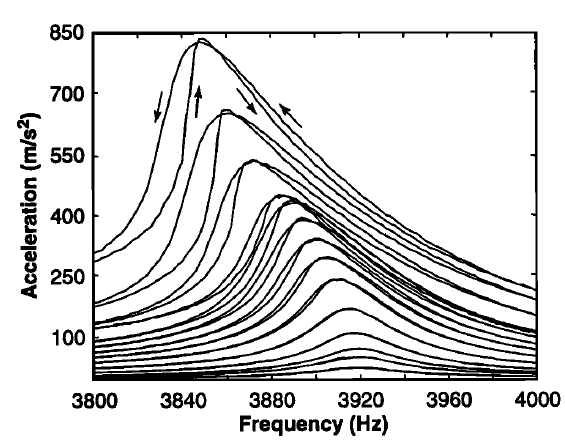
Real rocks show the same “leaning peak”: higher drive produces a shifted, skewed resonance curve. Figure adapted from Ten Cate & Shankland (1996).
5.3 Up–down differences: the curve depends on which way you sweep
A classic experimental trick is to sweep frequency upward, then sweep it downward, and compare the two curves. In many rocks, they do not match.
In the model, this is a visible “fingerprint” of memory: because contacts have finite switching times, the internal state does not reset instantly. If the dwell time $ \Delta t $ is short compared with the slowest contacts (set by $ \tau_{\\max} $), then the system carries history from one frequency step to the next.
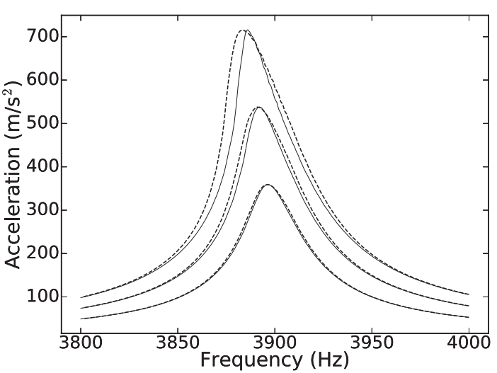
An important (and testable) point: for weak to moderate nonlinearity, the model predicts that these up–down differences should shrink when you sweep slowly, i.e. when $ \Delta t \gtrsim \tau_{\max} $.
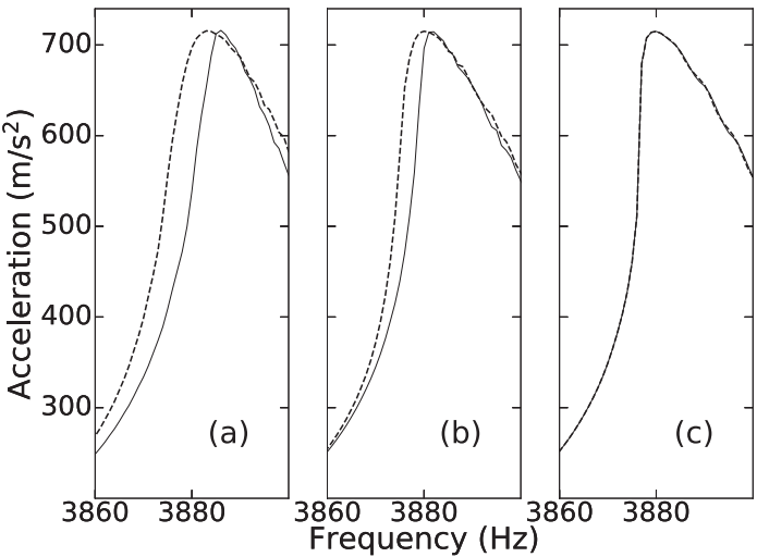
Up–down differences are strong for fast sweeps, but can fade for slow sweeps when memory has time to relax.
5.4 Hysteresis loops: the rock “lags” behind the loading cycle
Resonance sweeps are one way to reveal nonlinearity. Another is to keep the frequency fixed and simply cycle the strain up and down, the way DAET does: a low-frequency “pump” gently stretches and compresses the sample, while a high-frequency ultrasonic probe tracks how stiffness (or wave speed) changes within each cycle.
In a perfectly elastic, memoryless material, stiffness would be a single-valued function of strain: at the same strain you would measure the same stiffness, whether you are loading or unloading. But in granular rocks—and in the model—contacts switch state with finite rates. That means the internal damage-like variable $ N_o(t) $ cannot keep up instantly. The result is a loop: on the way back, the rock follows a different path.
The important point is that we do not have to add hysteresis by hand. It appears naturally once the stiffness depends on an evolving internal population of open/closed contacts with rate-dependent switching.
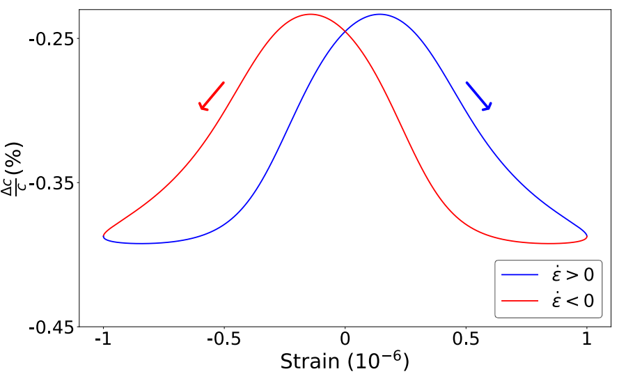
Predicted modulus–strain “butterfly” loops under cyclic strain: stiffness during unloading differs from stiffness during loading because $ N_o(t) $ lags behind the strain cycle.
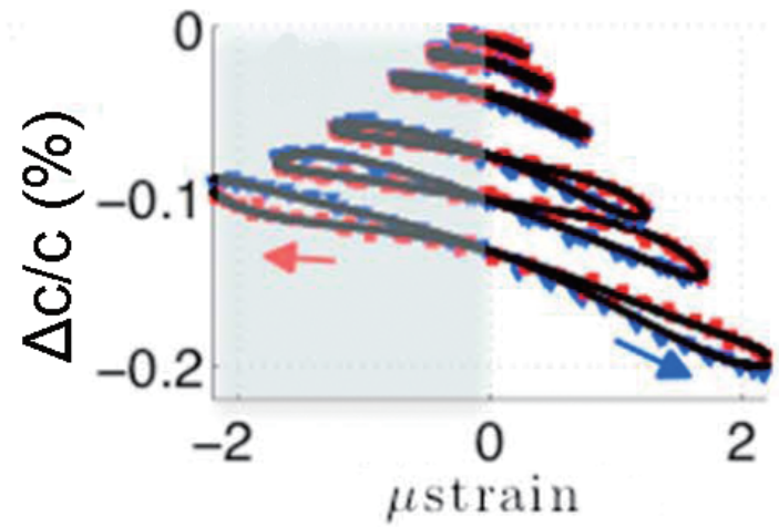
DAET measurements show the same signature: wave speed (and inferred stiffness) traces a loop rather than a single curve, indicating fast nonlinear hysteresis. Adapted from Rivière et al. (2015b).
- The loop’s width reflects delay (lag) between strain and contact-state evolution.
- The loop’s area is a compact measure of hysteresis: bigger area means stronger history dependence during the cycle (often interpreted as nonlinear dissipation / irreversible micro-slips at contacts).
- The “butterfly” shape comes from asymmetry: closing under compression is not a mirror image of opening under extension.
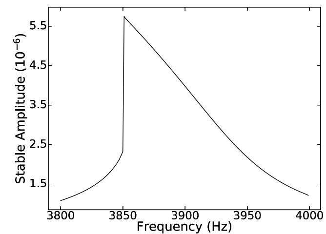
5.5 Cliffs: when resonance “snaps” between two stable states
Sometimes the resonance curve does something more dramatic than a gentle skew. It develops a near-vertical segment—the famous “cliff”—where a tiny frequency change produces a large jump in response.
In the model, this happens in a strongly nonlinear regime when the feedback loop becomes powerful: large response $ \rightarrow $ more contact opening $ \rightarrow $ lower stiffness $ \rightarrow $ resonance shifts in a way that reinforces the large response. Mathematically, this corresponds to a bifurcation: in a certain frequency band there can be two different stable steady states for the same drive frequency. The system follows one branch until it becomes unstable, then it jumps to the other—hence the cliff.
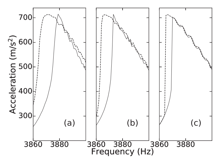
Strong nonlinearity can generate cliffs (jump behaviour) and persistent up–down differences near the jump.
At high drive, rocks can show jump-like features in frequency sweeps—an experimental “cliff”.
Earlier we said that up–down differences can come from slow dynamics: if the contacts relax slowly, the rock “remembers” where it just was, so an upward sweep and a downward sweep don’t match. But our model shows something even more striking: the largest up–down difference can survive even for slow sweeps, especially right at the “cliff”.
The reason is a bifurcation—a standard nonlinear-systems idea that also appears in the classic Duffing oscillator. In plain language, a bifurcation means: for the same driving frequency, the system can settle into two different stable steady states.
In our contact picture, the “state” is the fraction of open defects, $ N_o $ (you can think of it as a damage-like variable: larger $ N_o $ means more contacts are open and the sample is softer). We make this idea very clear by doing a simplified calculation: they temporarily turn off the time evolution and ask a steady question:
“If we drive at one fixed frequency and just wait long enough, what equilibrium value of $ N_o $ do we end up with?” And crucially: “Does that equilibrium depend on where we started (the initial damage $ N_{oi} $)?”
For moderate nonlinearity, the answer is boring (in a good way): the system has one stable equilibrium at each frequency. No matter what initial condition you start from, you converge to the same $ N_o $. In that regime, slow sweeps tend to erase up–down differences.
For strong nonlinearity, the answer changes: there is a frequency band where two stable equilibria exist. That is the bifurcation band. Inside it, the final state depends on your starting point, $ N_{oi} $—which is exactly what a frequency sweep changes. In other words, the rock can “lock into” one of two stable stiffness (damage) states.
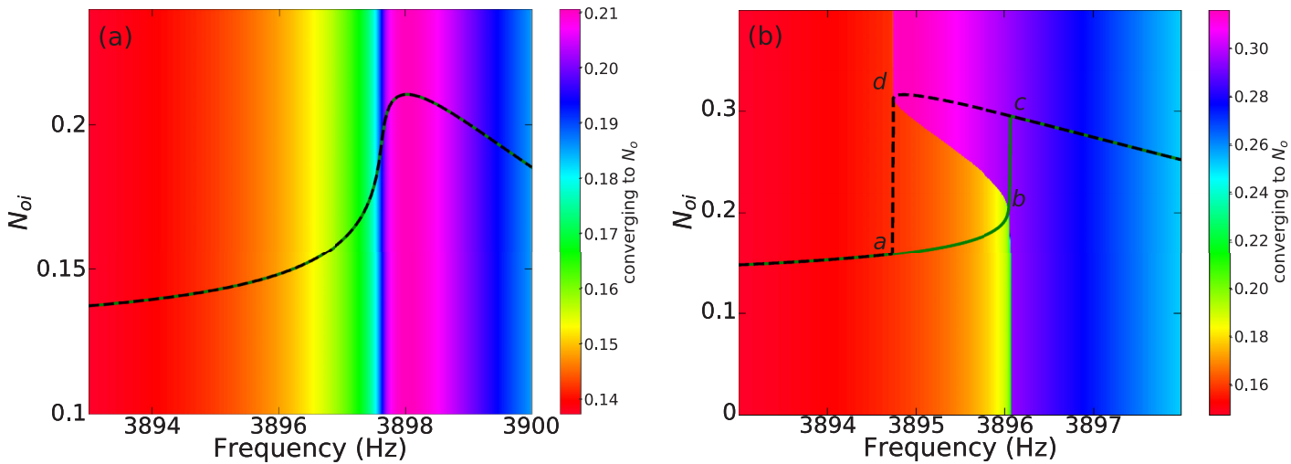
Over a certain frequency range, there are two stable equilibrium branches for $ N_o $ (two possible steady states), separated by an unstable branch. Which stable state you end up on depends on the initial condition $ N_{oi} $. This is the key mechanism behind persistent up–down differences at the cliff.
This also explains why slow sweeps don’t always fix the problem. If the system has only one stable equilibrium at each frequency, then sweeping slowly gives the internal state time to settle, and up-sweep and down-sweep curves can converge. But if there are two stable equilibria, then “waiting longer” does not force the system onto a single unique answer. It merely gives it time to settle onto one of the two—and which one depends on the direction you came from.
Technically, this is the same qualitative mechanism behind Duffing “jump” phenomena: strong nonlinearity can make the response curve fold over; increasing nonlinearity further produces multiple steady solutions, where the middle branch is unstable. In the thermodynamic model, the feedback loop (large vibration $ \rightarrow $ more contact opening $ \rightarrow $ softer modulus $ \rightarrow $ shifted resonance) provides the nonlinearity needed to create that fold and bifurcation.
Hence, practical takeaways are that up–down differences can have two origins:
- Memory / slow dynamics (rate effect): tends to shrink for slow sweeps, when $ \Delta t \gtrsim \tau_{\max} $.
- Bifurcation / multiple stable steady states (true nonlinearity): can persist even for slow sweeps, especially at the cliff.
6) Conclusion: A Unified, Contact-Based Explanation of Nonlinear Rocks
This project set out to answer a deceptively simple question: how can microstrain-level vibrations produce such large, history-dependent changes in the elastic response of granular rocks? Our main result is a compact, thermodynamics-based contact model that treats grain contacts / microcracks as bistable elements (open vs. closed) with rate-dependent switching. When this internal state is coupled to a realistic resonance-measurement protocol (“hold–measure–step”), it reproduces the core experimental signatures of nonlinear elasticity in granular solids within one consistent framework. What we built is a minimal model in which dynamic strain biases defect energies, defects switch states over activation barriers, the evolving open fraction $ N_o(t) $ changes stiffness $ Y(t) $, and that stiffness feeds back into the driven resonance.
The model explains the following laboratory obervations of nonlinear elasticity in a unified way:
- Amplitude-dependent resonance shifts and asymmetric peaks: the resonance “leans” because stiffness evolves most strongly near resonance, so the natural frequency drifts during the sweep.
- Fast hysteresis (DAET/NRUS loops): loading and unloading differ because $ N_o(t) $ lags behind the strain cycle when switching is rate-limited.
- Slow dynamics and near log-time recovery: a broad distribution of barrier energies produces a wide spectrum of relaxation times, so recovery is not controlled by a single time constant and can appear logarithmic over long windows.
- “Cliffs” (jump behaviour) and persistent up–down differences: in strong nonlinearity, the coupled contact–oscillator system admits multiple stable steady states (a bifurcation band), so sweep direction can matter even when the sweep is slow.
These observations and underlying mechanisms matter beyond the lab: The same ingredients that control bench-top resonance experiments—contact-level metastability, rate effects, and broad relaxation spectra—also provide a natural physical language for field observations: post-seismic velocity drops and recovery, time-lapse changes during injection/production, and other crustal transients where “damage-like” compliance evolves with forcing and then heals gradually.
This work should also enable other research possibilities:
- Account for fluids, pressure, and temperature: extend the energy landscape so switching rates depend on effective stress and pore pressure, enabling direct links to saturation changes and reservoir operations.
- Bridge to frictional fault physics: couple contact-state evolution to rate-and-state friction to connect resonance/DAET observations to fault-zone transients and triggered slip.
- Embed in monitoring/inversion: use the model as an interpretable forward operator to infer $ N_o(t) $ or $ Y(t) $ from time-lapse wave-speed data (e.g., crosswell, ambient noise, or DAS).
- A targeted “two-equilibria” experiment: drive at a fixed frequency inside the predicted bifurcation band, prepare different initial conditioning states, and test whether two distinct stable outcomes emerge—an unambiguous signature of genuine multistability rather than rate effects alone.
Many “mysterious” nonlinear rock phenomena can be interpreted as the macroscopic footprint of a large population of micro-contacts exploring a biased energy landscape—some responding quickly, others retaining memory for a long time.
Related: Xun Li, A unified interpretation of nonlinear elasticity in granular solids – Master’s thesis, Colorado School of Mines.
References
- Gassenmeier, M. (2016). Observation of dynamic processes with seismic interferometry. PhD Thesis, Universität Leipzig, Leipzig.
- Guyer, R.; Johnson, P. (2009). Nonlinear Mesoscopic Elasticity: The Complex Behaviour of Rocks, Soil, Concrete. Wiley‑VCH.
- Guyer, R.A.; McCall, K.R.; Van Den Abeele, K. (1998). Slow dynamics, memory and nonlinear elasticity. Geophysical Research Letters, 25(9), 1585–1588. DOI: 10.1029/98GL00818.
- Johnson, P.A.; Zinszner, B.; Rasolofosaon, P.N.J. (1996). Resonance and elastic nonlinear phenomena in rock. Journal of Geophysical Research, 101(B5), 11553–11564. DOI: 10.1029/96JB00323.
- Landau, L.D.; Lifshitz, E.M.; Kosevich, A.M.; Pitaevskii, L.P. (1986). Theory of Elasticity. Elsevier.
- Li, X.; Sens‑Schönfelder, C.; Snieder, R. (2018). Nonlinear elasticity in resonance experiments. Physical Review B, 97, 144301. DOI: 10.1103/PhysRevB.97.144301.
- Li, X. (2018). A unified interpretation of nonlinear elasticity in granular solids. Master’s thesis, Colorado School of Mines.
- Lyakhovsky, V.; Hamiel, Y.; Ampuero, J.-P.; Ben‑Zion, Y. (2009). Nonlinear damage rheology and wave resonance in rocks. Geophysical Journal International, 178, 910–920. DOI: 10.1111/j.1365-246X.2009.04207.x.
- Okubo, K.; Delbridge, B. G.; Denolle, M. A. (2024). Monitoring velocity change over 20 years at Parkfield. Journal of Geophysical Research: Solid Earth, 129, e2023JB028084. DOI: 10.1029/2023JB028084.
- Rivière, J.; Shokouhi, P.; Guyer, R.A.; Johnson, P.A. (2015a). Simple measurements of dynamic acousto‑elasticity: Protocols and modeling. Journal of Geophysical Research: Solid Earth, 120, 1587–1600. DOI: 10.1002/2014JB011491.
- Rivière, J.; Shokouhi, P.; Guyer, R.A.; Johnson, P.A. (2015b). A set of measures for the systematic classification of the nonlinear elastic behavior of disparate rocks. Journal of Geophysical Research: Solid Earth, 120, 1587–1604. DOI: 10.1002/2014JB011718.
- Snieder, R.; Sens‑Schönfelder, C.; Wu, R. (2017). The time dependence of rock velocities explained by a non‑recoverable nonlinearity. Geophysical Journal International, 208, 1–7. DOI: 10.1093/gji/ggw389.
- TenCate, J.A.; Shankland, T.J. (1996). Nonlinear resonance and hysteresis in rock. Geophysical Research Letters, 23, 3019–3022. DOI: 10.1029/96GL02884.
- TenCate, J.A.; Smith, E.; Guyer, R.A. (2000). Universal slow dynamics in granular solids. Physical Review Letters, 85, 1020–1023. DOI: 10.1103/PhysRevLett.85.1020.
- TenCate, J.A. (2011). Slow dynamics of consolidated granular media. Pure and Applied Geophysics, 168, 2211–2219. DOI: 10.1007/s00024-011-0280-6.
- Vakhnenko, O.O.; Vakhnenko, V.O.; Shankland, T.J. (2005). Nonlinear behavior of rocks under compression and tension. Physical Review B, 71, 174103. DOI: 10.1103/PhysRevB.71.174103.