What Thousands of Induced Earthquakes Taught Us about Hydraulic Diffusivity and Aseismic Slip at the UK Geothermal Test Site (Rosemanowes, Cornwall).
In the early 1980s, engineers drilled into hot granite beneath a Cornish quarry and began pumping in water at high pressure. The idea was simple and bold: turn “hot dry rock” into a man‑made geothermal reservoir. As the water forced its way through the rock, the subsurface cracked, creaked, and slipped—sometimes loudly enough to register as tiny earthquakes, and sometimes in complete silence.Decades later, we went back to this classic experiment at Rosemanowes with fresh eyes and modern analysis tools. We studied 5,184 microearthquakes triggered during the main stimulation phase, most of which are far too small to be felt by humans at the surface, but rich with information about how the rock responded to injection. By comparing how much the rock deformed overall with how much of that deformation showed up as seismic shaking, we could ask a simple but fundamental question:
When we inject fluid into the subsurface, how much of the resulting deformation becomes earthquakes—and how much slips by quietly, without a sound?
The answer at Rosemanowes was striking. Only a tiny fraction of the injected strain was released seismically; most of the deformation was effectively silent. At the same time, the expanding “cloud” of event locations revealed that the reservoir was far from uniform. Seismicity spread much more easily up and down than sideways, pointing to a strongly anisotropic (direction‑dependent) flow field with exceptionally high vertical permeability. Our research draws a solid picture that fluid exploits pre‑existing fractures: some slipping in shear and radiating seismic waves, many more opening and creeping aseismically to form efficient vertical pathways for flow.
Related: Li, Main & Jupe, Induced seismicity at the UK ‘hot dry rock’ test site for geothermal energy production (2018).
1) Site and Geological Background
The Rosemanowes geothermal test site sits in a granite quarry on the Carnmenellis pluton in southwest England, a short drive from Falmouth in Cornwall. At the surface it looks fairly ordinary – a worked quarry face, heathland, farm tracks – but beneath it lies one of the UK’s best‑characterised blocks of hot crystalline rock. This made Rosemanowes an ideal natural laboratory for “hot dry rock” (HDR) geothermal research in the late 1970s and 1980s.
The Carnmenellis granite is part of the Cornubian batholith, a chain of granitic bodies stretching from Dartmoor in Devon all the way to the Isles of Scilly (Exley & Stone, 1964; Searle et al., 2024). Gravity surveys indicate that the granite beneath Rosemanowes extends to at least 10 km depth (Bott et al., 1958), forming a thick, relatively homogeneous block of low‑porosity, low‑permeability rock. Thermal measurements showed a favourable geothermal gradient: at depths of 2–3 km the rock temperature exceeds 80–100 °C, warm enough to be interesting for heat extraction but still technically drillable with conventional rigs for the time.
Crucially, the granite is tight: it contains very little connected pore space. Fluids don’t flow easily through the intact matrix. Instead, most permeability comes from natural fractures and joints – planes of weakness formed during the granite’s cooling and its long subsequent tectonic history. Borehole image logs at Rosemanowes revealed two main sets of steeply dipping joints: one trending roughly NW–SE (often called Set 1), and another roughly NE–SW (Set 2; Baria et al., 1984b, 1984e). These pre‑existing joint sets would later prove central to understanding how the injected fluid moved and how the induced seismicity was organised.
The regional stress field in southwest England is also relatively well constrained from hydraulic tests and mining data. At Rosemanowes, the maximum horizontal compressive stress (σH) trends approximately NW–SE and exceeds the minimum horizontal stress (σh) by several tens of megapascals at ~2 km depth (Baria et al., 1983). This means that some of the subvertical joints are already close to failure in shear: a modest increase in pore pressure along those planes can effectively “unclamp” them and trigger slip. From a geomechanics perspective, Rosemanowes offers a relatively simple but informative configuration: a thick, stiff granite body, a well‑defined ambient stress field, and a known fracture network.
The HDR concept tested here was to turn this otherwise impermeable hot rock into a useable geothermal reservoir by engineering a connected fracture system at depth. The programme drilled at least two deep wells into the granite: RH12, an inclined injection well reaching ~2 km, and RH11, a production well used to recover a fraction of the injected water (Baria et al., 1984a). Rather than relying on explosive stimulation, the operators injected water at elevated pressures to encourage slip and opening along existing fractures and to enhance connectivity between them. Over time, they alternated between high‑rate “stimulation” periods and lower‑rate circulation phases, during which water was pumped from RH12, flowed through the stimulated fracture network, and was recovered at RH11.
One of the most innovative aspects of the Rosemanowes project was its microseismic monitoring. In the early 1980s it was far from standard practice to run dense downhole seismic arrays and systematically catalogue thousands of microearthquakes. At Rosemanowes, a network of vertical‑component and three‑component accelerometers was cemented in shallow boreholes, up to ~300 m deep, directly into the granite host rock (Baria et al., 1984c). These were complemented by calibration shots and vertical seismic profiling (VSP) surveys to refine the local velocity model (Baria et al., 1984d). Because the reservoir sits within a relatively uniform granitic block that outcrops at the surface, ray paths from microearthquakes to the sensors traverse mainly granite, allowing a comparatively simple half‑space velocity model with station delays to be used.
This careful experimental design paid off. During the main creation and development phase of the reservoir (Phase 2A), the network detected and located 5,184 induced microearthquakes, with magnitudes down to about Mw ≈ −1 (and smaller, closer events below this threshold). Each event was recorded on multiple downhole stations, enabling reasonably precise hypocentre locations and spectral estimates of scalar seismic moment (Andrews, 1986). For the time, this was an exceptionally rich induced‑seismicity data set – one that could only later be fully exploited as analysis methods matured (e.g. Dinske & Shapiro, 2013; Shapiro, 2015).
In short, Rosemanowes combined three things that are rarely available together: a simple geological setting, a well‑controlled hydraulic experiment, and a high‑quality microseismic catalogue. That combination makes it an ideal natural laboratory for exploring how fluid injection, fracture networks, and induced seismicity interact – and for asking how much of a geothermal reservoir’s deformation is noisy, and how much happens in near‑silence.
Location on the Carnmenellis granite, part of the Cornubian batholith – a low‑porosity, low‑permeability pluton extending to >10 km depth (Bott et al., 1958; Baria et al., 1984c).
2) Injection and Production with Seismicity Response
The Rosemanowes experiment was, at heart, a controlled plumbing exercise in very hard rock. Water was pumped down the injection well (RH12) and, some of it at least, came back up the production well (RH11). The first figure shows how this played out over time: the injected volume (VI) climbs steadily as operators push more water into the granite, while the produced volume (VP) lags behind. The gap between those two curves is the net stored volume, VN = VI − VP –– effectively, how much extra water is being held somewhere in the subsurface rather than coming back to the surface. What’s striking is how large that gap becomes. Even after production starts, the net storage keeps growing, telling us that the reservoir is acting as a very compliant sponge: it can take in a lot of water without forcing it all back out.
Then we track how the tiny earthquakes respond to these operational changes. When injection rates are high, the cumulative seismic moment (a measure of total seismic “work” done by all the microearthquakes) rises in steps. During “shut‑in” periods, when the production well is closed and flow pauses or changes, seismicity often quietens down – sometimes almost completely. The annotations – “stimulation”, “shut‑in”, “aseismic” – help link what the pumps are doing at the surface to how the rock is responding at 2 km depth. Most of the time, despite large changes in injected volume, the seismic response is surprisingly modest.
Cumulative injection, production, shut-ins, and stimulations. The widening gap between injection and production shows how much fluid is retained in the subsurface.
Periods of high‑rate stimulation coincide with bursts of microseismicity, whereas shut‑ins and some circulation phases are relatively quiet or even almost aseismic.
To make this more quantitative, we compared how fast seismic moment accumulated with how fast net fluid volume was increasing, using 30‑hour time windows. This gives us an apparent shear modulus, μap, and from that a strain partition factor η – the fraction of total deformation that shows up as earthquakes. The third figure summarises the key result: η is tiny, about 10−4, meaning only around 0.01% of the injected strain was released seismically. And as injection continued, μap didn’t stay constant. Instead, it showed a clear step‑like drop once the net stored volume reached roughly 70,600 m³. In other words, as the reservoir filled and the fracture system became better connected, the rock increasingly accommodated additional deformation silently – through elastic expansion, aseismic slip, and crack opening – rather than by generating more microearthquakes. The seismic response actually decelerated, even as more and more water was being stored at depth.
As net injected volume grows, the apparent shear modulus μap drops in a step, implying that additional deformation is increasingly taken up aseismically rather than by earthquakes.
3) How Seismogenic “Noisy” is the Reservoir?
Once we know when and where the microearthquakes happened, the next question is: how big were they, and what does that say about the state of the reservoir? Seismologists have a simple but powerful way to summarise this, called the Gutenberg–Richter law. It says that small earthquakes are much more common than large ones, and that the relationship between frequency and size can be captured by a straight line on a log–linear plot. The slope of that line is the famous b‑value. For global tectonic earthquakes, b is typically around 1. At Rosemanowes, using thousands of events reliably detected down to about Mw ≈ −1.0, we found a much steeper slope: b ≈ 2.3. In practical terms, this means the sequence is heavily dominated by very small events, with relatively few larger ones. Laboratory and field studies link high b‑values to low “stress intensity” on the largest fractures: the system is not strongly focused onto one big fault, but rather spread across many smaller cracks in a relatively compliant, well‑buffered volume.
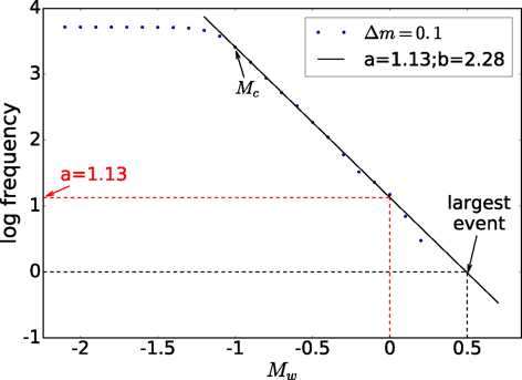
The frequency–magnitude curve is steep (b ≈ 2.3), meaning many tiny events and very few larger ones – a statistical fingerprint of low stress concentration on the largest fractures.
A high b‑value tells us the shape of the earthquake size distribution, but it doesn’t tell us how “trigger‑happy” the reservoir is overall. For that, we use another metric: the seismogenic index, Σ, introduced by Shapiro and colleagues. Σ measures how many earthquakes you get per unit of injected fluid volume, for a given magnitude threshold. High Σ means a reservoir that responds to injection with lots of seismicity; low Σ means that most of the deformation is taken up silently. At Rosemanowes, we tracked how the number of events above various magnitude cut‑offs grows with net injected volume and used this to estimate Σ. For a threshold around Mw ≈ −0.8, we obtained Σ ≈ −4.2 – low compared to many geothermal projects worldwide, and much closer to values reported for some unconventional hydrocarbon reservoirs. This is entirely consistent with what we saw in the strain partition analysis: very little of the injected strain shows up as earthquakes, and the system’s overall susceptibility to induced seismicity is modest despite substantial fluid volumes.
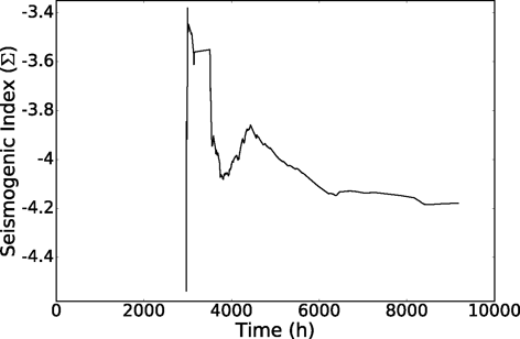
As net injected volume increases, the number of events above a given magnitude grows slowly. A low Σ ≈ −4.2 indicates that Rosemanowes is relatively “quiet” per cubic metre of water injected, with most deformation occurring aseismically.
4) How Does the Fluid Really Move? From Simple Diffusion to Channelled Flow
When you inject water into hot, fractured granite, you might imagine the pressure spreading outwards like dye in a still pond: smoothly, symmetrically, and at a predictable rate. In that ideal world, pore pressure relaxes in a uniform, isotropic medium and the “activation front” for induced earthquakes – the distance out to which events are triggered – grows like r ∝ t1/2. This is the classic diffusion picture many models start from.
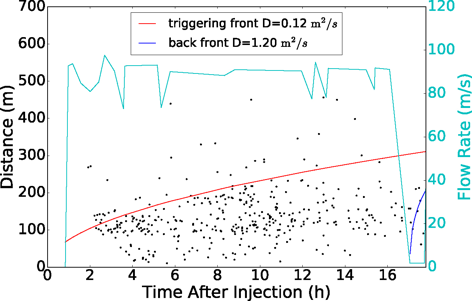
Distances of individual events from the injection point (dots) compared with a reference curve behaving like r ∝ t1/2. Early and late deviations from this smooth envelope hint at heterogeneous, evolving permeability rather than simple, uniform diffusion.
At Rosemanowes, the data tell a more interesting story. If we track how far each microearthquake is from the injection point and how that distance changes with time, we can sketch an envelope around the expanding cloud of events – the so‑called “triggering front”. The first plot below shows these distances as dots, along with a reference curve behaving like r ∝ t1/2. Early on, many events fall outside this smooth envelope; later, some parts of the cloud seem to stall at preferred distances, hinting at specific fractures or zones that keep reactivating. This already suggests that a simple, uniform diffusion model is not capturing what the reservoir is actually doing.
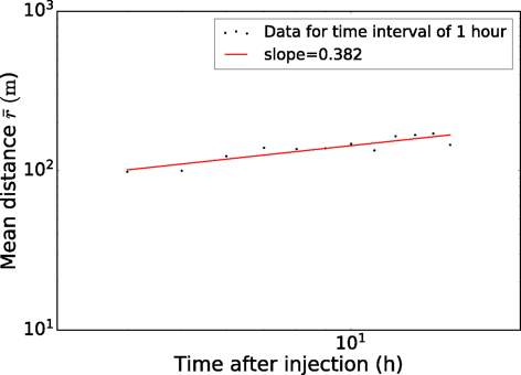
The mean distance of events grows roughly as r ∝ t0.382, significantly slower than the 1/2 exponent expected for classical diffusion – consistent with anisotropic channeling of flow through a fracture network dominated by vertical pathways.
To go beyond that first look, we averaged event distances in 1‑hour windows and examined how the mean distance grows with time on log–log axes. In a purely Fickian (textbook) diffusion process, the slope of that line should be 0.5. Instead, we find a slope of about 0.38. This slower‑than‑expected growth is a hallmark of non‑Fickian diffusion: the fluid and pressure are not spreading out evenly in all directions, but are being steered and bottlenecked by the fracture network and evolving permeability. In other words, the reservoir behaves less like a uniform sponge and more like a network of preferential pathways and barriers.
We can push this idea further by fitting a three‑dimensional surface to the outer edge of the seismic cloud. If the medium were isotropic, that surface would be a sphere. Instead, the best fit at Rosemanowes is a stretched ellipsoid: relatively short in one horizontal direction, somewhat longer in the perpendicular horizontal direction, and dramatically elongated vertically. From this geometry we can back out effective hydraulic diffusivities along the three principal axes:
- D11 ≈ 0.01 m²/s (minor horizontal axis, ~NE)
- D22 ≈ 0.03 m²/s (intermediate horizontal axis, ~NW)
- D33 ≈ 1.6 m²/s (major axis, vertical)
Time‑lapse of induced events at Rosemanowes, with a best‑fit ellipsoid outlining the evolving boundary of the seismic cloud. The pronounced vertical elongation of the triggering front reflects the highly anisotropic hydraulic diffusivity of the stimulated reservoir.
The above vedio shows the evolution of induced seismicity during Phase 2A at Rosemanowes in three dimensions. Each point marks a microseismic event at its recorded hypocentre, coloured by time and scaled by seismic moment. As time progresses, the cloud of events expands away from the injection zone, revealing a strongly anisotropic growth pattern. Superimposed on the seismicity cloud is a best‑fit three‑dimensional ellipsoid that tracks the outer boundary of the events (the “triggering front”). If the rock mass behaved as a homogeneous isotropic medium, this boundary would be approximately spherical. Instead, the fitted surface is markedly elongated in the vertical direction and compressed along one horizontal axis, consistent with a homogeneous but anisotropic hydraulic diffusivity tensor in the principal coordinate system:
The vertical component exceeds the horizontal components by almost two orders of magnitude, implying that once stimulation begins the reservoir either develops or reactivates an extremely efficient vertical fluid conduit. Pressure and fluid diffuse up and down much more readily than laterally, and the triggering front inherits this strong anisotropy. Together with the statistical and structural analyses presented elsewhere, this supports a picture of injection fluid exploiting a pre‑existing, stress‑aligned fracture network: a subset of fractures slip seismically to form the microearthquake cloud, while many more open or creep aseismically, linking into a vertically oriented plumbing system that governs the advance of the pressure front.
5) Fracture Networks, Stress, and Focal Mechanisms
So far we have treated the microearthquake cloud mainly as a set of distances from the injection well. But the shape of that cloud in three dimensions, and how it relates to the fractures and stresses in the rock, is just as revealing. When we plot the epicentres in map view, colour‑coded by time, they fill out an elongated ellipse around the injection point. Most events sit neatly inside this envelope; only a few outliers to the northwest poke beyond it, perhaps hinting at local channels or patches that were already close to failure before injection began. In cross‑section, the picture becomes even clearer: the microseismicity forms a vertically stretched ellipsoid, much taller than it is wide. This echoes what we saw in the flow analysis – the reservoir is far from isotropic, and vertical connectivity is especially strong.
Downhole image logs and core data tell us that this cloud of seismicity is not forming in a featureless block of granite. Instead, it is threading its way through a pre‑existing joint network. Two main families of steeply dipping joints dominate: a NW–SE trending set (Set 1), and an orthogonal NE–SW set (Set 2). Independent hydraulic tests and mining data show that the present‑day maximum horizontal stress, σH, also trends roughly NW–SE – almost exactly along the major horizontal axis of the seismic ellipse. In other words, the direction in which seismicity spreads most easily on the horizontal plane is the same direction in which the rock is being squeezed the hardest, and the same direction picked out by one of the main joint sets. This alignment is a strong clue that we are seeing the stress field and the fracture architecture working together to guide both flow and failure.
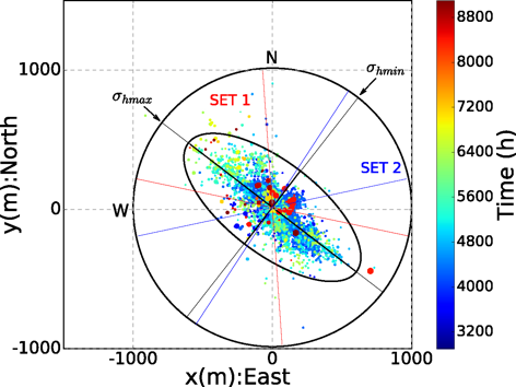
The induced events fill an elongated ellipse whose long axis aligns with the maximum horizontal stress and with the dominant joint set. Only a few outliers lie beyond the envelope, hinting at possible fluid channels or particularly sensitive patches.
When we look at vertical cross‑sections, the vertical extent of activity really stands out. The induced earthquakes occupy a tall, column‑like volume extending hundreds of metres above and below the injection depth. This reinforces the idea from the diffusivity analysis that a highly permeable vertical structure – or a bundle of structures – is being activated. The combination of horizontally aligned maximum stress and vertically dominant permeability suggests a “ladder” geometry: stress controls which subvertical joints are primed for slip, while vertical connections allow pressure to migrate up and down far more readily than sideways.
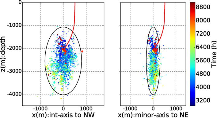
Depth sections show a strongly elongated seismic cloud, with the longest axis vertical. This geometry is consistent with a vertically connected fracture system providing efficient up‑ and downward fluid pathways.
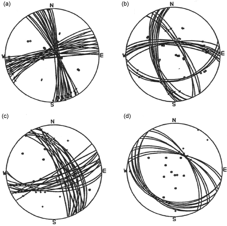
Most focal mechanisms are strike‑slip, with a smaller number showing normal‑faulting components. The preferred strike‑slip planes line up with Set 1 joints and the maximum horizontal stress, indicating shear reactivation of pre‑existing fractures rather than the creation of entirely new faults.
Source mechanism analysis – the “beach ball” diagrams familiar from earthquake bulletins – adds another layer of evidence. By stacking and inverting waveforms from clusters of microearthquakes, we obtain composite focal mechanisms that describe the average fault orientation and slip style. At Rosemanowes, these solutions are predominantly double‑couple, strike‑slip types, with a lesser contribution from normal‑faulting events. The strike of the preferred slip planes tends to lie at an angle of about 20–40° to the maximum horizontal stress, exactly where Coulomb friction theory predicts shear reactivation should be easiest. Crucially, one nodal plane in the dominant mechanisms is subparallel to the NW–SE Set 1 joints, while the orthogonal Set 2 planes are more strongly clamped by the present‑day stress field. This points to slip occurring mainly on Set 1 fractures, with Set 2 joints playing more of a passive role as potential opening or linkage features.
Time‑lapse view of induced seismicity and operations during Phase 2A. The top row shows three 2‑D slices through the reservoir along its principal axes: plan view (x–y), and two vertical sections (x′–z and y′–z) aligned with the intermediate and minor horizontal axes of the best‑fit ellipsoid. Each dot is a microearthquake, coloured by occurrence time and scaled by seismic moment, plotted relative to the injection point (yellow square) and the inclined injection well (red line). The bottom panel tracks cumulative injection, production, and net stored volume over the same time window. Together, these panels show how the seismic cloud expands into an elongated, vertically dominated ellipsoid while the reservoir progressively fills and the balance between injection and production shifts.
The above vedio makes the 3‑D structure of the Rosemanowes reservoir much easier to see. As time advances, the coloured microearthquakes light up around the end of the injection well and then spread outwards, first near the wellbore and then along preferred directions picked out by the fracture network and stress field. In plan view, the cloud fills an elongated ellipse whose long axis aligns with the maximum horizontal stress and the dominant joint set. In cross‑section, the activity stretches vertically, revealing the tall, column‑like geometry of the stimulated volume. Meanwhile, the lower panel shows how injection, production, and net storage evolve in step with this growth: as more water is pumped in and only part of it is recovered, the reservoir inflates elastically, fractures open and creep, and the seismic cloud gradually maps out the portion of the rock mass that has been brought into hydraulic communication — much of it deforming almost silently.
6) A Consistent Triggering Mechanism
By this point we’ve looked at the Rosemanowes experiment from several angles: how much fluid went in and out, how many earthquakes were triggered, how their sizes are distributed, and how the seismic cloud expands in 3‑D. The natural next question is: what is the actual mechanism tying all of this together? In other words, what is the rock doing at the fracture scale when we inject water?
The source‑mechanism analysis – the “beach ball” diagrams built from clusters of microearthquakes – provides a crucial constraint. Most events have double‑couple, strike‑slip focal mechanisms, with a smaller number showing normal‑faulting components. The preferred slip planes are steeply dipping and oriented about 20–40° to the maximum horizontal stress, σH, which is exactly the range where Coulomb friction theory predicts that shear reactivation is easiest. One of these nodal planes lines up with the NW–SE Set 1 joints identified in the borehole image logs, while the orthogonal Set 2 joints carry higher normal stress and are less likely to slip in shear. This points strongly to the recorded microseismicity being generated by shear slip on optimally oriented pre‑existing Set 1 joints, not by entirely new fractures cutting through intact granite.
At the same time, several lines of evidence tell us that shear slip is only the tip of the iceberg. The strain partition factor, η, is around 10−4, meaning that only about 0.01% of the total deformation shows up as earthquakes. The volumetric strain implied by the net injected volume and the size of the seismic ellipsoid is on the order of 10−3 – large enough that, in principle, a lot more seismic strain could have been released. Instead, most of the deformation is taken up aseismically: through elastic expansion of a very compliant fracture system, slow creep on fractures that never quite “let go” dynamically, and opening of tensile cracks that radiate little or no detectable seismic energy. As injection and circulation proceed, the apparent shear modulus drops in a step‑like fashion, and η decreases, indicating that the system becomes increasingly efficient at deforming silently rather than by generating additional microearthquakes.
The conceptual model in the figure below pulls these threads together. In the present‑day stress field, the NW–SE Set 1 joints are favourably oriented for shear, while the NE–SW Set 2 joints are more tightly clamped. When pore pressure increases along Set 1, the effective normal stress on those planes is reduced, promoting both seismic and aseismic shear slip. That slip has an important side effect: it tends to pull apart the orthogonal Set 2 joints in tension, especially where the two sets intersect. These opening segments act as tensile conduits – vertical and subvertical pathways that dramatically enhance permeability and allow fluid and pressure to move up and down much more easily than sideways.
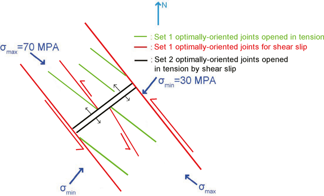
Schematic view of the fracture network at Rosemanowes. Red lines indicate shear slip on NW–SE‑striking Set 1 joints, optimally oriented in the present‑day stress field (σmax ≈ σH). Green segments represent tensile fractures opening parallel to σmax, often at intersections where shear on Set 1 pulls apart NE–SW‑striking Set 2 joints (black). This coupled shear‑and‑opening process creates vertically connected fluid pathways, explains the strong vertical permeability and anisotropic diffusion inferred from the seismic cloud, and accounts for why only a tiny fraction of the total deformation is radiated seismically.
In this view, the induced seismicity at Rosemanowes is the audible part of a much larger deformation process. The earthquakes we record come mainly from shear reactivation of a specific family of steep joints (Set 1), which are optimally oriented in the in‑situ stress field. Their slip, both seismic and aseismic, helps to pry open the intersecting Set 2 joints and other tensile cracks, stitching together a vertically oriented, high‑permeability network. This network can store large volumes of injected fluid, transmit pressure efficiently, and deform in a predominantly aseismic way. The result is a reservoir that looks highly active in terms of fluid movement and strain, but relatively quiet in terms of felt seismicity – a key insight for understanding and managing the risks of geothermal stimulation in similar fractured crystalline rocks.
7) Implications for Geothermal Operations and Risk
Rosemanowes offers a useful reminder that “more fluid” does not automatically mean “more earthquakes”. The reservoir experienced substantial deformation – volumetric strains on the order of 10−3 – yet only about 0.01% of that strain was released seismically. Most of the work went into elastic expansion, aseismic slip, and tensile opening of fractures. In other words, a jointed, compliant granite can quietly absorb a great deal of pressure and fluid without necessarily generating large or frequent felt events. For geothermal developers and regulators, this is both reassuring and challenging: reassuring because it shows that engineered reservoirs can deform largely silently, challenging because standard seismic monitoring only captures a very small fraction of what is actually happening underground.
The Rosemanowes data also show that the seismic response can decelerate with time. As injection progressed and the circulation phase began, the apparent shear modulus and strain partition factor dropped in a step, suggesting that once a well‑connected fracture system was established, further pressurisation tended to be taken up more aseismically. The seismogenic index Σ is low and decreases with ongoing injection, again indicating a reservoir that becomes less seismically responsive per unit volume of water. At the same time, fluid flow clearly did not behave like simple, uniform diffusion: induced events mapped out a vertically elongated ellipsoid and a non‑Fickian triggering front, pointing to strong vertical channeling of flow through a fracture network aligned with the stress field. All of this underscores that the details of the fracture system and stress state matter at least as much as the raw injection volume.
What does this mean in practice for managing induced seismicity at geothermal sites, in Cornwall and elsewhere? A few key lessons emerge:
- Most deformation can be silent. Low strain partition factors (η) and a low seismogenic index (Σ) imply that large volumetric strain can accrue with only a small seismic footprint. Relying on microseismicity alone will underestimate how much the reservoir has actually deformed. Whenever possible, seismic monitoring should be combined with pressure, flow, and possibly geodetic data to get a fuller picture of reservoir response.
- Expect anisotropic flow. Rosemanowes demonstrates that pre‑existing joint sets and the in‑situ stress field can focus flow into highly anisotropic patterns, with vertical permeability orders of magnitude higher than horizontal. In design and risk assessment, we should expect fluids to be funnelled preferentially along certain directions – particularly vertically – and not to spread out evenly in all directions. This has implications for where pressure fronts may reach critically stressed faults, and how far from the injection well seismicity might be triggered.
- Seismic response can decelerate. The step‑like drop in apparent shear modulus with increasing net injected volume at Rosemanowes suggests that, in some reservoirs, the seismic response may be strongest early in stimulation and then weaken as a compliant fracture network becomes fully engaged. This is different from a “runaway” or near‑critical scenario often feared in public discussions. Operational strategies that allow time for the reservoir to adjust – staged injections, pauses, and careful ramp‑up of rates – may help encourage this kind of self‑buffering behaviour, though this will be site‑specific.
- Monitoring priorities. The Rosemanowes case highlights how important it is to characterise the fracture system and stress field ahead of time. Joint‑set orientations, in‑situ stresses, and likely vertical connectivity should be core inputs to any induced‑seismicity risk assessment. Downhole imaging, stress testing, and early‑stage microseismic data can all be used to refine models of which fractures are most likely to slip seismically and where vertical channels might form. These models, in turn, should feed into real‑time traffic‑light systems for adjusting injection rates or temporarily shutting in wells if seismicity begins to concentrate in unfavourable locations or on critically stressed structures.
In summary, the Rosemanowes experiment shows that induced seismicity in HDR and EGS projects is not simply a matter of “how much water” but of where that water goes and how it interacts with the existing fracture fabric and stress field. Minimising induced seismicity means designing and operating reservoirs with these structural and mechanical subtleties in mind – aiming for fracture networks that carry most of the deformation aseismically, while watching closely for signs that pressure fronts are approaching large, well‑oriented faults that could respond more noisily.
References
- Andrews, D. J. (1986). Objective determination of source parameters and similarity of earthquakes of different size. In S. Das, J. Boatwright, & C. H. Scholz (Eds.), Earthquake Source Mechanics (pp. 259–267). American Geophysical Union. https://doi.org/10.1029/GM037p0259
- Baria, R., Hearn, K., Lanyon, G., & Batchelor, A. (1984a). Camborne School of Mines geothermal energy project: Hydraulic results (Technical report). Camborne School of Mines.
- Baria, R., Hearn, K., Lanyon, G., & Batchelor, A. (1984b). Camborne School of Mines geothermal energy project: Jointing (Technical report). Camborne School of Mines.
- Baria, R., Hearn, K., Lanyon, G., & Batchelor, A. (1984c). Camborne School of Mines geothermal energy project: Microseismic results (Technical report). Camborne School of Mines.
- Baria, R., Hearn, K., Lanyon, G., & Batchelor, A. (1984d). Camborne School of Mines geothermal energy project: Seismic velocity structure (Technical report). Camborne School of Mines.
- Bott, M. H. P., Day, A. A., & Masson-Smith, D. (1958). The geological interpretation of gravity and magnetic surveys in Devon and Cornwall. Philosophical Transactions of the Royal Society of London A, 251(992), 161–191. https://doi.org/10.1098/rsta.1958.0013
- Dinske, C., & Shapiro, S. A. (2013). Seismotectonic state of reservoirs inferred from magnitude distributions of fluid-induced seismicity. Journal of Seismology, 17, 13–25. https://doi.org/10.1007/s10950-012-9292-9
- Exley, C. S., & Stone, M. (1964). The granitic rocks of South-West England. Proceedings of the Geologists’ Association, 75(3), 305–322. https://doi.org/10.1016/S0016-7878(64)80002-0
- Li, X., Main, I., & Jupe, A. (2018). Induced seismicity at the UK ‘hot dry rock’ test site for geothermal energy production. Geophysical Journal International, 214, 331–344. https://doi.org/10.1093/gji/ggy135
- McGarr, A. (2014). Maximum magnitude earthquakes induced by fluid injection. Journal of Geophysical Research: Solid Earth, 119, 1008–1019. https://doi.org/10.1002/2013JB010597
- Parotidis, M., Shapiro, S. A., & Rothert, E. (2004). Back front of seismicity induced after termination of borehole fluid injection. Geophysical Research Letters, 31, L02612. https://doi.org/10.1029/2003GL018987
- Searle, M. P., Shail, R. K., Pownall, J. M., Jurkowski, C., Watts, A. B., & Robb, L. J. (2024). The Permian Cornubian granite batholith, SW England; Part 1: Field, structural, and petrological constraints. GSA Bulletin, 136(9–10), 4301–4320. https://doi.org/10.1130/B37457.1
- Shapiro, S. A. (2015). Fluid-Induced Seismicity. Cambridge University Press. https://doi.org/10.1017/CBO9781139051132